Originally published on Efficiently (Substack)
A few years ago, I gave a talk at Spark Summit 2020 about File Formats covering Avro, ORC, and Parquet. I received numerous questions about that topic, responding point-to-point, leaving the knowledge confined to those forums alone.
That isn’t helpful for most people. This post aims to fix that.
In this series, I’ll outline the primitives of this topic and then explore the hands-on details.
Problem
In the efficiency space, minimizing “work” is key. Whether work requires compute, network, or storage, “the goal of efficient data usage is to get the most accurate answer in the fastest and cheapest way possible.”
File Formats help data practitioners store their data in ways that minimize work. When you think of a file format, you may think of extensions like .xlsx, .pdf, .pptx. Similarly, technologies like Parquet, Avro, and ORC serve this purpose.
Background / Example Data
A partition is a logical segment of data. In the big data world, this usually means a piece of a larger dataset. For our purposes, I’m going to use an example dataset below.
This dataset has 3 columns (Column A, Column B, and Column C) and 4 rows (Row 0, Row 1, Row 2, and Row 3).
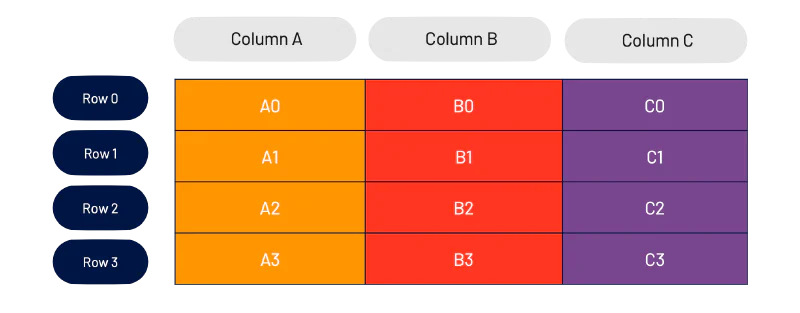
This table should look familiar — something you’ve seen in Excel, Pandas, etc. Let’s take this example further and split the individual elements into their own logical “pieces.”
We can refer to each “cell” by its “<column><row>.” For example, the second row in Column B is called B1.
Storage
Background
Data is stored on hard disks in what is called a block. A block is the minimum amount of data read during any read operation.
Blocks function like a suitcase. When checking a bag on a trip, you pay the same price regardless of how full or empty your suitcase is. It’s optimal to fill your suitcase with as many relevant objects as possible, in as easy a way to find as possible.
Extending this analogy: packing unnecessary stuff isn’t great. Bringing too many suitcases (unless strictly necessary) also isn’t great. Inside the suitcase, you want to “group” similar things together — each pair of socks should be next to each other in the same suitcase, rather than split across different ones.
In hard drives, these insights apply. Reading unnecessary data is expensive. Reading fragmented data is expensive. Random seeks are expensive as well.
Our goal is to lay data out in a manner optimized for our workflows.
Row-wise Storage
In database land, the common way to store data used to be row-wise. It’s pretty easy to understand why. Most people think about datasets as a list of rows.
Taking our dataset above, let’s store this in a row-wise method.
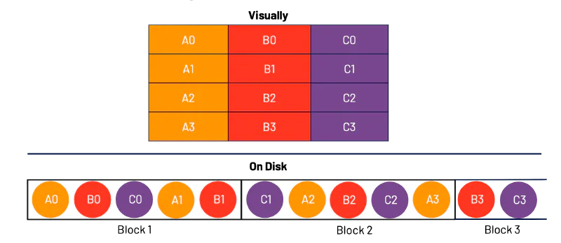
I have taken each row in order and packed as much of the rows as I can into a block, before moving to the next block.
This method works great when the goal is to read the data sequentially. All that’s required is a simple linear scan of the block in order. It doesn’t work as well if, for example, you want to only look at Column C. In that case, you’re required to read all of the block (i.e., read all of the data) and filter down to Column C.
This is row-wise storage methodology.
Columnar (Column-wise) Storage
Column-wise storage takes the opposite approach and orients around columns.
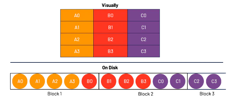
As you can see, we first take the entire column, pack it into a block, and then move onto the next column.
This method works great when the data is read in a columnar way (i.e., one column at a time). It doesn’t work well if, for example, you want to reconstruct Row 0. In that situation, you’d need to read all of the data and filter down to the elements that make up Row 0.
Now, we’re in a dilemma — one approach seems to favor a row-oriented workflow, one approach seems to favor a column-oriented workflow. Luckily for us (and Goldilocks), there’s a middle ground.

Hybrid Storage
A hybrid storage model gives us the best of both worlds. First, we group a fixed number of Rows together and then further group that by columns. We segment these and call these “Row Groups” (at least in the Parquet terminology).
In this example, we first selected two rows — Row 0 and Row 1. We then grouped those rows by column, and inserted them into our first Row Group.
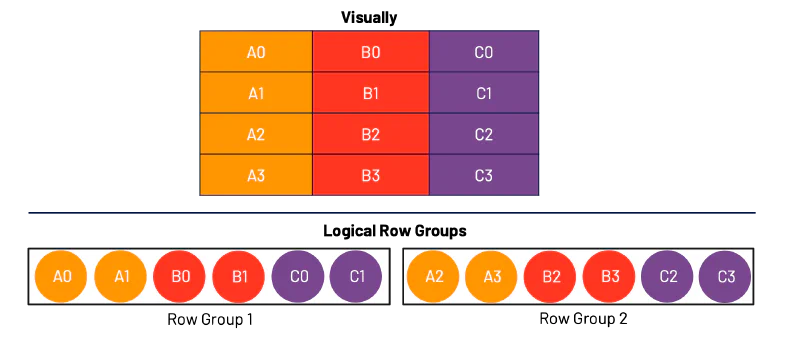
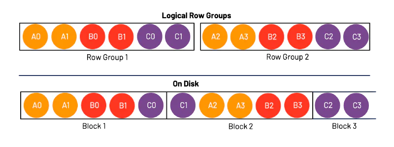
I called these logical Row Groups because this is more of how we should be thinking about them, rather than how they may necessarily end up on disk.
This representation of data is actually immensely powerful. It allows us to optimize our workflows for both row-oriented and column-oriented operations.
Let’s talk about how this works.
In the case of a row-oriented workflow, let’s say you want to recreate Row 2. To do this, you would simply need to look at Block 1 and Block 2. If you were operating in a Columnar storage model, you would need to look at Block 1, Block 2, and Block 3. You’ve saved a whole Block!
In the case of a column-oriented workflow, let’s say you want to recreate Column B. In this case, you would simply need to look at Block 1 and Block 2. If you were operating in a Row-wise storage model, you would need to look at Block 1, Block 2, and Block 3. You’ve once again saved a whole Block!
Our examples used very small data, you can imagine how this extrapolates further with larger datasets.
Data Workflows
Throughout this post, I’ve referred to my data workflows as “row oriented” or “column oriented.” Luckily for us, the big data community has come up with some terminology that should help bring these two workflows to life.
OLTP
Online Transaction Processing (OLTP) workloads generally involve larger amounts of short queries/transactions. These tend to be more focused on processing than analytics and as such have more data updates and deletions. Roughly — we can consider OLTP workflows as “row oriented” workflows.
OLAP
Online Analytical Processing (OLAP) workloads are more analysis than processing focused. As such, there tends to be more analytical complexity per query and fewer CRUD transactions. Roughly — we can consider OLAP workflows as “column oriented” workflows.
Conclusion
Using data efficiently relies on using all levels of the “data stack” (storage, network, compute) efficiently. Reducing the amount of unnecessary data read during a query process can have compounding effects on the speed and efficiency of your analytics process.
In subsequent parts of this series, I’ll be digging more into the details of how everything we have covered thus far can be applied in analytics workloads.